In many testing problems, we want to test many hypotheses at a time, e.g.
Test for in linear regression.
Test whether each of single nucleotide polymorphisms (SNPs) is associated with a given phenotype (e.g. diabetes/schizophrenia)
Test whether each of website tweaks affects user engagement
Setup: . . (e.g. ) commonly, . Goal: return an accept/reject decision for each .
. Problem: Even if all true, probably have . Classical solution: control family-wise error rate (FWER) . I.e. .
1.1 Familywise Error Rate
Problem: even if all are true, might have .
Example
, . .
Is this a problem? Yes. If all attention will be focused on the (false) rejections and non on the (correct) non-rejections.
Classical solution is to control the familywise error rate (FWER):
If hypothesis tests independent, we can use (Sidak correction)
Then
For small , , so Sidak doesn't improve much on Bonferroni.
Example
. Coordinate-wise multiple testing . How large does Bonferroni threshold have to be?
Turns out for large .
Test .
3 Testing with Dependence
Bonferroni isn't much worse than Sidak, e.g. : . But when tests are highly dependent, can often do much better.
Example (Scheffe's S-method)
, for ()
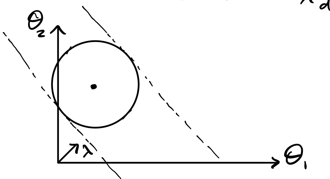
Reject if . (Because ) Controls FWER: Can view as deduction from confidence region .
4 Deduced Inference
Given any joint confidence region for , we may freely assume and "deduce" any and all implied conclusions without any FWER inflation.
Deduction is often a good paradigm for deriving simultaneous intervals.
We say are simultaneous confidence intervals for if .
Example (Simultaneous intervals for multivariate Gaussian)
Assume , is known, . Let be the upper- quantile of .
Note we could have instead constructed an elliptical confidence region but then the intervals would be conservative.
Example (Linear regression)
observations, variables, design . Estimate . Then , where . distribution of is fully known.
Assume WLOG that . Let denote upper- quantile of . Then are simultaneous confidence intervals for (compute by simulation), then